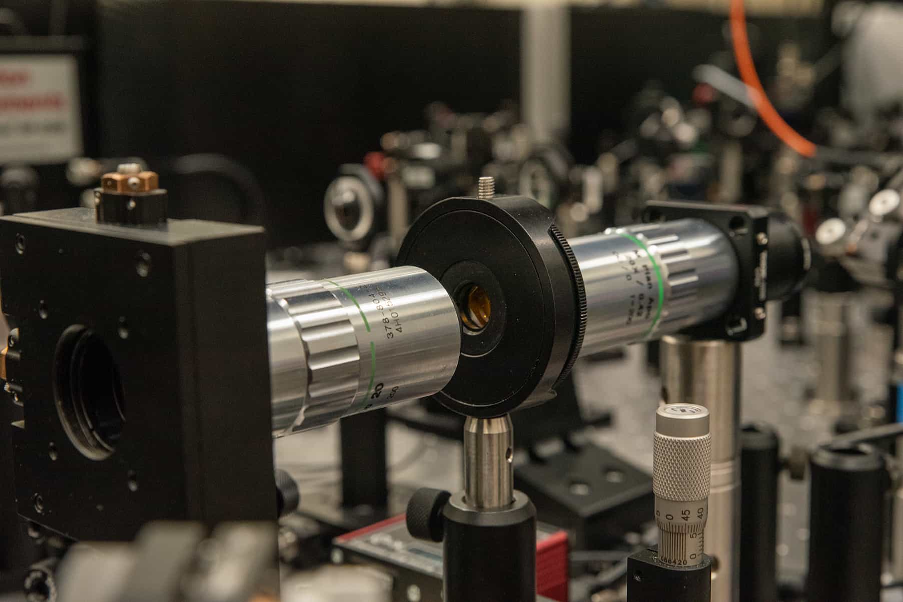
An optics experiment at NIST (illustrative; not a quantum-eraser setup) · Image credit: B. Hayes/NIST · Public domain (NIST, US government work)
Quantum22 min read
The quantum eraser: single photons, a double slit, and what “erasing” really means
Tag which slit each photon took and the stripes vanish. Erase the tag and they come back, but only in half the light. That half is the whole trick, and nothing travels back in time.
Companion video: The quantum eraser ↓
Contents
- How dim is “one photon at a time”?
- Dots that add up to stripes
- What “which-path information” really is
- What the eraser actually does
- Do it later: the delayed-choice version
- Partial tags, partial stripes
- Is any of this actually quantum?
- Open questions
- How sure are we?
- What the video simplified
- Further reading
- References
Picture a lecture demo you may have seen online. A green laser shines through two narrow slits onto a camera. The laser is turned down so far that the camera records only single bright dots, each one a photon, a particle of light, appearing at random places. Wait long enough and the dots crowd into stripes. Then someone puts a small polarizing filter over each slit, the two turned at right angles (a polarizing filter passes light wiggling in only one direction, like polarized sunglasses), and the stripes disappear. A third filter goes in front of the camera, and the stripes come back. Because that third filter seems to wipe out the record of which slit each photon used, the setup is called a quantum eraser.
The usual telling comes with big words: the photon knows it is being watched, or a later choice reaches back in time. None of that is needed, only bookkeeping about which photons end up in which pile. The physics is textbook-solid. (A warning up front: the tabletop demo also has an ordinary, pre-quantum explanation; near the end we come back to what makes the research versions genuinely quantum.)
How dim is “one photon at a time”?
Light comes in indivisible lumps of energy called photons. A detector never registers half a photon: it either clicks or it doesn’t Reference 4. Each photon of green light carries so little energy that even a feeble beam holds enormous numbers of them.
Take a beam of one nanowatt, a billionth of a watt. It still delivers about 2.7 billion photons every second. They travel at the speed of light, so on average they are about 11 cm apart along the beam, and a 1-meter tabletop setup holds about nine of them at any moment (before the slits, which block most of them). That is not “one at a time.”
11 cm
AVERAGE GAP BETWEEN PHOTONS · 1 nW GREEN BEAM
At one picowatt, “one at a time” is fair, with two footnotes.
A dimmed laser does not hand out photons on a schedule. Its photons arrive at random, like raindrops on a roof, so now and then two arrive close together Reference 5. Even at one picowatt, when the setup holds a photon at all, about 1 time in 220 it holds two or more.
There is a deeper problem too. Dots alone don’t show that light comes in lumps: a detector clicks one dot at a time even when a smooth wave falls on it, because the detector itself works in lumps. So physicists use a sharper test. Put a beam splitter (a half-silvered mirror that sends each photon one way or the other at random) in front of two detectors. A single photon can only go one way, so it never makes both click at once. A classical wave, the smooth, endlessly divisible wave of pre-quantum physics, splits in two, so both detectors sometimes click together by chance. Dimmed laser light makes them click together exactly as often as a steady classical wave would Reference 5. No classical wave can do better than that; real single photons do. The laser’s light is still made of photons, but they arrive at random, so this test cannot tell them apart from a wave. A dimmed laser shows the build-up beautifully, but cannot by itself rule out a classical wave.
That needs a source that really emits one photon at a time. In 1986 Grangier, Roger and Aspect, in Orsay, France, used atoms that emit photons in pairs, so detecting one announced its partner. These photons made both detectors click together only about a fifth as often as any classical wave could (not zero, because photons from other atoms occasionally slipped in). In an interferometer (which splits light along two paths and recombines them), the same light made interference fringes, the physicists’ word for stripes, with almost perfectly dark bands: more than 98 % contrast Reference 4.
For physicistsPhoton flux, Poisson statistics and the anticorrelation test3 equations · ~3 min
For a continuous beam of power and wavelength , the mean photon flux and the mean number of photons inside a length of beam are
At nm, J. So nW gives and , while pW gives a mean spacing m, and an empty 1 m stretch 99 % of the time (computed in calc/photon-flux.ts; refractive index of air neglected, losses at the slits ignored).
An attenuated laser is a coherent state, so photon numbers are Poissonian and the fraction of non-empty windows holding two or more photons is (0.45 %, about 1 in 220, at ).
The discriminating test is the anticorrelation parameter used by Grangier, Roger and Aspect,
with the number of trigger windows, the counts behind each output of a beam splitter and the coincidences. Any semi-classical model (classical field, quantized detectors) obeys by the Cauchy–Schwarz inequality; an ideal one-photon state gives ; Poissonian light gives . With an atomic-cascade source heralded by the first photon of each pair, Grangier et al. measured at their optimal gate width, their most significant violation (more than 13 standard deviations), and saw fringe visibility above 98 % with the same source in a Mach–Zehnder interferometer Reference 4. With a single NV center, Jacques et al. found for single-photon pulses and for faint laser pulses (95 % confidence intervals) Reference 5. Strictly, rules out semi-classical models under their stated assumptions.
Dots that add up to stripes
The stripes are called interference: the pattern you get when two waves overlap, adding where crest meets crest and cancelling where crest meets trough. Light from the two slits travels slightly different distances to each point on the screen, so the two contributions alternately reinforce and cancel, and the screen shows bright and dark bands, or fringes.
The strange part is that this happens with one photon at a time. Each photon arrives as a single dot, and no single dot shows a stripe. But the dots avoid the dark bands and pile up in the bright ones: the pattern exists only in the statistics, yet depends on both slits being open. In the language of quantum mechanics, each photon passes through the slits in a superposition of the two paths, a combination of both that is not the same as one or the other Reference 1. This double personality, a wave when it travels and a dot when it lands, is often called wave–particle duality.
Matter does it too. Electrons, the particles in every atom, make the same stripes. In a 1989 experiment at Hitachi, Akira Tonomura and colleagues fitted an electron microscope with a fine wire that splits each electron’s wave in two, an electron version of a double slit. About 1,000 electrons arrived per second, and at a large fraction of the speed of light each was on average 150 km behind the one before, while the whole path was only 1.5 m long: there was very little chance of two being inside at once. Clear fringes emerged from about 70,000 single dots Reference 6. (With light, the idea is old: in 1909 G. I. Taylor exposed a photographic plate to very dim light for three months and found the pattern as sharp as ever Reference 7.)
Two more words before the main sequence. Light is a wave whose electric field wiggles from side to side as it travels; the direction of the wiggle is its polarization. A polarizer lets through only one wiggle direction; light wiggling at 45° to it gets through half the time. In what follows, the laser’s light starts out wiggling diagonally.
Step by step
From scattered dots to stripes, and what the eraser really brings back
Twelve photons have arrived, each a single dot at a random-looking place. (Every dot is drawn from the equations that predict the pattern.)
Figure: Twelve dots scattered across an empty screen behind a double slit. No pattern is visible.
After 400 photons the dots are clumping. The bar chart counts how many landed in each narrow strip: regular bumps are emerging.
Figure: About 400 dots. Below the screen, a bar chart of counts across the screen starts to show regular bumps.
At 6,000 photons the stripes are unmistakable, about 2.1 mm apart for this illustrative setup. The orange line is the prediction for light that could have come through either slit, and the dots follow it.
Figure: 6,000 dots forming clear vertical stripes about 2.1 mm apart. A predicted curve with sharp peaks and zeros sits on the bars.
Now tag the slits: the diagonal light leaving the left slit is turned to wiggle horizontally (H), at the right slit vertically (V). Transparent crystal plates (wave plates) can do this without absorbing light. Same number of photons, same total light, but the stripes are gone: a smooth hump.
Figure: Slits now marked H and V. 6,000 new dots form a single smooth hump with no stripes. The predicted curve has no zeros.
Add the eraser: a polarizer at 45°, halfway between horizontal and vertical. It lets through 50 % of the photons, and those show stripes again. Nothing new was added; half the photons were removed.
Figure: A polarizer at plus 45 degrees is added before the screen. About half the dots remain, and they form stripes again.
Where did the other half go? Turn the polarizer to −45°. These are the photons a +45° filter blocks, and they show stripes too, but shifted: their bright bands fill the previous dark bands. Physicists call these anti-fringes.
Figure: The polarizer is turned to minus 45 degrees. The other half of the dots appear, forming stripes shifted so their peaks sit where the previous troughs were.
Put the two halves back together. Fringes plus anti-fringes add up to the smooth, stripe-free hump. The eraser never brought the pattern back for all the light. It sorted the photons into two piles, each with its own stripes.
Figure: Both halves shown together in two shades. Their stacked counts form the smooth hump of the tagged experiment; the orange sum curve has no stripes.
The last step is the heart of the matter. Tags that only turn the wiggle destroy no light: some light from the bright bands now lands in the dark bands, flattening the stripes into the smooth hump. (Absorbing filters, as in the lecture demo, also remove light, but the stripes vanish the same way.) And the eraser did not repair the stripes either. Set at 45°, it passes exactly half the light, and for that half the tag tells you nothing about the slit. The blocked half carries the shifted stripes; add the halves and you get back the stripe-free pattern Reference 1Reference 2.
For physicistsThe intensities behind the figure5 equations · ~4 min
In the far field (or the focal plane of a lens), with slit width , center-to-center separation , wavelength and slit–screen distance , define and . The single-slit amplitudes are , and with identical polarization
the form also given by Kim et al. for their coincidence rate Reference 2. With orthogonal, lossless tags ( on slit 1, on slit 2; e.g. a half-wave plate on each slit, or on one slit if the input is ) the cross term vanishes: , with the same integral as . Absorbing and polarizers on light polarized at 45° would multiply this by (Malus’s law). A linear polarizer at angle from transmits , so
The visibility behind the polarizer is , and its sign distinguishes fringes from anti-fringes. The transmitted fraction is , where is the normalized integral of ; for any real double slit , so exactly one half is transmitted at every angle (ideal polarizer).
For quarter-wave-plate tags (fast axes at ±45° to the input polarization, the arrangement of Walborn et al.’s Sec. III, turning slit-1 and slit-2 light into opposite circular polarizations Reference 1) and a linear polarizer acting on the slit photon itself at , both are projected with equal magnitude and opposite phases:
so the fringes return at full visibility for every but shift by of a fringe spacing (sign convention-dependent). When the polarizer acts instead on an entangled partner, as in Walborn et al.’s experiment, projecting the partner (their Eqs. 8–9) leaves conditional marker states with overlap , so the coincidence visibility is with fixed fringe positions (their Eq. 16; calc/double-slit.ts). The figure uses the illustrative values nm, m, m, m: fringe spacing mm, first diffraction zero at mm, nine bright fringes in the central lobe (the fifth orders fall on envelope zeros). Positions are seeded inverse-CDF samples; each tagged photon’s ±45° outcome is drawn with probability (calc/buildup.ts).
What “which-path information” really is
The tags in the scrolly are a kind of which-path information: any physical record, stored anywhere, that could in principle tell you which slit a photon went through. Here the record is the photon’s own polarization. Light from the left slit wiggles horizontally, light from the right slit vertically, and a suitable filter could sort the two perfectly.
Why does that kill the stripes? Stripes need the two waves to cancel each other in the dark bands: a crest from one slit meeting a trough from the other. But a horizontal wiggle and a vertical wiggle move in different directions. A left–right push cannot undo an up–down push, so the two waves simply add their brightness everywhere, and there are no dark bands.
Notice what this does not require. Nobody has to look at the polarization. The stripes vanish because the information exists in the light; as Walborn and colleagues put it in their 2002 analysis, it is enough that the which-path information is available Reference 1. That is why talk of consciousness or “being watched” misses the point.
An old explanation says that measuring the path must jostle the particle and scramble the stripes. That isn’t what happens here: the tags barely disturb where the light goes Reference 1. Following a 1982 proposal by Marlan Scully and Kai Drühl, physicists recognized that the stripes can disappear simply because the path has become linked to a separate record Reference 8Reference 1. In the most striking versions, the record is shared with a second photon, linked to the first by entanglement: a connection that makes the two photons’ results correlated however far apart they are, and whether you measure their wiggles as horizontal-or-vertical or as one-diagonal-or-the-other.
What the eraser actually does
The eraser is a polarizer set at 45°, diagonally between horizontal and vertical. Horizontal and vertical light have equal chances of getting through a diagonal filter, and every photon that does get through comes out wiggling diagonally, identical to all the others. Nothing is left to tell which slit it came from, so for those photons interference returns.
The price is that the filter blocks the other half, and those blocked photons are not random leftovers. A filter at −45° would instead keep that other group, and it shows shifted stripes. Why shifted? Measured along the +45° direction, the horizontal and vertical wiggles both point “forward.” Along −45°, one of them points “backward,” which turns every crest of that slit’s wave into a trough, so bright and dark bands swap.
Walborn’s team saw this with a real double slit. Their tags were quarter-wave plates, crystal plates that turn a straight wiggle into a corkscrew-like circular one, clockwise for one slit and anticlockwise for the other. With the plates in place the stripes vanished, apart from a small residue from imperfect alignment. Their eraser, a polarizer acting on a second photon born together with the first (how that works is explained below), gave fringes with the polarizer at one angle and anti-fringes with it turned by 90°; the two averaged to roughly the stripe-free pattern Reference 1.
So “erasing” is a strong word. Count every photon, including the blocked ones, and the total pattern never changes; the tabletop camera shows stripes only because the eraser threw away the half with the opposite stripes. The eraser really sorts the photons into two groups, each showing stripes.
Do it later: the delayed-choice version
In the tabletop version the eraser acts on the same photon that hits the screen. In the research versions, the which-path record is shared with a partner photon, and the eraser acts on the partner. A special crystal splits one laser photon into an entangled pair, a process called down-conversion Reference 1Reference 2.
In Walborn’s experiment the pair had linked polarizations: whenever the partner wiggles vertically, the slit photon wiggles horizontally, and the other way round. One photon went through the slits, tagged with wave plates that turn horizontal and vertical light into corkscrews of opposite handedness, to a detector; the other went to a polarizer and a second detector. If the partner wiggles vertically, the slit photon’s corkscrew turns one way for the left slit and the other way for the right; if the partner wiggles horizontally, the roles swap. So knowing both polarizations reveals the slit Reference 1. The eraser is a diagonal polarizer on the partner. A partner that gets through comes out diagonal, its horizontal-or-vertical wiggle gone, and with it the key to the slit photon’s corkscrew. Every slit photon still lands on its detector; the partner’s result only decides which pile it is filed in. Slit photons whose partners passed show stripes; with the filter turned by 90°, the slit photons matched with partners that pass show shifted stripes. Matching does not create stripes; it reveals which photons belong together. Electronics typically pair detections arriving within a few billionths of a second, allowing for any known delay Reference 9; this is called coincidence counting. When the team lengthened the partner’s path so the slit photon was detected first (with the polarizer set in advance; the authors note no real choice was made), the results were the same: in their words, the order of detection is not important Reference 1.
A more elaborate version, by Yoon-Ho Kim, Marlan Scully and colleagues, published in 2000, works differently Reference 2. There the double slit sits in the laser beam before the crystal, so the pair can be born in the crystal behind the left slit (spot A) or behind the right slit (spot B); in fact it is born in a superposition of both. The first photon goes to a detector moved step by step across the pattern. Its partner enters a maze of beam splitters: some routes lead to detectors that see only A or only B, revealing the birth spot; others mix the two, losing the record. Its route was decided at a beam splitter about 7.7 nanoseconds (7.7 billionths of a second) after the first photon was detected, by chance, not by a person. When the first photons were sorted by their partners’ fates, one group showed fringes, another anti-fringes, and the which-path groups none Reference 2.
It is tempting to read this as the future reaching back. Look at the bookkeeping. The first photons, taken all together, never show stripes: fringes plus anti-fringes plus no-fringes add up to no stripes. Kim’s team checked: the first detector’s own count, taken alone, was flat across the scan Reference 2. The stripes appear only after sorting the earlier records with information about the partners, brought over by ordinary means, no faster than light. Looking only at the first detector’s counts, you can never tell what was done to the partners.
A major review concludes that these experiments can mimic an influence of the future on the past but need no signals into the past Reference 3. As the physicist Sean Carroll puts it, nothing went backwards in time Reference 10.
A different question remains: could each photon settle in advance whether to behave as a wave or a particle, matching whatever will be measured? To test that, the choice must be made in a way the photon could not know about. In experiments in Vienna (the partner sent through 55 m of optical fiber) and in the Canary Islands (over a 144 km open-air link), a quantum random-number generator, a device that uses a quantum process to make truly unpredictable coin flips, decided how to measure the partner. In Vienna, and in one of two timing arrangements on the islands, no light-speed signal could connect that choice with the other photon’s passage through its interferometer. The results matched quantum mechanics: a photon that is definitely a wave or definitely a particle would need some influence faster than light Reference 11. (Over the island link, background clicks had to be subtracted.)
That test used entangled pairs. An older single-photon test, proposed by the physicist J. A. Wheeler, is weaker. A single photon, with no partner, enters an interferometer whose second beam splitter is put in or taken out at the last moment: in, the two paths recombine and interfere; out, each detector reveals the path Reference 12. In 2018 Rafael Chaves and colleagues showed that its results can be faked by a photon carrying a simple hidden “instruction card” Reference 13. Experiments in 2019 used a slightly modified test and ruled such cards out, as long as the card holds just one of two values (a single bit), like the photon’s choice between two paths Reference 14Reference 15. None of this touches the main point: no signal goes back in time.
For physicistsDelayed erasure without retrocausality3 equations · ~3 min
Write the slit photon and the which-path marker (a partner photon, or the polarization degree of freedom) as
with orthogonal marker states, . In Walborn et al. the marker states are joint states of both photons’ polarizations (their Eqs. 8–9); in Kim et al. the path is the birth region A or B, shared by both photons through their momentum correlation.
Measuring the marker in the conjugate basis yields, conditional on the outcome, the slit-photon state with probability each (for non-overlapping slit modes, ): fringes or anti-fringes. The unconditional state of the slit photon is
independent of which basis (if any) is chosen for the marker and of when that measurement happens. This is the no-signalling property: the marginal screen distribution carries no information about the marker setting. Projectors on different subsystems commute, so detection order is irrelevant; conditional patterns appear only in coincidence data Reference 1Reference 2Reference 3. Walborn et al. call the “alter the past” reading an erroneous interpretation of the formalism Reference 1.
In Kim et al. the idler’s optical path to the beam splitters BSA and BSB, where the which-path or both-path “choice” is made, exceeded the signal’s path to D0 by ≃ 2.3 m, so the choice came at least 7.7 ns after the signal was registered (the arXiv preprint quoted ≃ 2.5 m to the detectors) Reference 2Reference 3.
Ma et al. made the choices space-like separated from the interference events; for the 144 km link (33 dB loss) agreement required background subtraction Reference 11Reference 3. Chaves, Lemos and Pienaar showed that Wheeler’s original interferometer scheme (not the entangled eraser), realized with single photons and a space-like separated random choice by Jacques et al. Reference 12, admits a simple classical causal model Reference 13. Device-independent tests of a modified scheme violated dimension witnesses, excluding non-retrocausal hidden-variable models of the quantum system’s dimension Reference 14Reference 15.
Interpretation. Ma, Kofler and Zeilinger read the state as a catalogue of knowledge Reference 3; Carroll gives an Everettian account Reference 10. Both make identical predictions.
Partial tags, partial stripes
Which-path information need not be all or nothing. If the right slit’s light is tilted short of vertical, you could use a filter to guess the slit right more often than not, and the stripes survive partly. The more reliably the path could be read, the fainter the stripes.
This trade-off has a precise form. Call the contrast of the stripes the visibility, from 0 (no stripes) to 1 (perfectly dark bands). Call the reliability of the path record the distinguishability: 0 means the best possible guess at the slit is a coin toss, 1 means it is always right, and in general the best guess is right a fraction (1 + distinguishability)/2 of the time. Quantum mechanics guarantees that the squares of the two can never add up to more than 1. If the best guess is right 80 % of the time (distinguishability 0.6), the stripes can have at most 0.8 visibility, since 0.6² + 0.8² = 1. Physicists derived this in the 1990s Reference 16, and experiments with single photons have since confirmed it Reference 3.
In the interactive below you meet a closely related trade-off with a different knob: you turn the eraser instead of the tags. At 0° the eraser passes only horizontal light, which all came from the left slit, so it reads the path perfectly and there are no stripes. (The interactive’s “path information” readout measures how well the slit can be guessed for the photons that get through.) At 45° the path information is gone and the stripes are perfect. In between, you get some of each.
Explorable · try it
Tag the slits, then try to erase the tag
Assumptions and simplifications
- Illustrative setup: green light at 532 nm, slits 50 µm wide and 250 µm apart, screen 1 m away; the screen shows ±12 mm. Not the parameters of a specific experiment.
- Ideal, lossless tags and polarizers, a perfect detector and perfectly steady, single-colored light. Real experiments see lower contrast.
- With no tags, both slits pass light of the same polarization (diagonal), so the eraser just dims everything equally and the stripes stay.
- The same random photons are reused for every setting. “Photons sent” counts photons reaching the eraser.
- “Path information” measures how well you could guess the slit for the photons that get through the eraser: 1 means always right, 0 means a coin toss.
Try the “Wave plates” option too, where the polarizer acts on the same photon. A straight polarizer at any angle passes equal amounts of clockwise and anticlockwise corkscrew light, so every angle erases the path and gives full-contrast stripes in the half that gets through, but turning it slides them sideways.
For physicistsComplementarity, quantified2 equations · ~2 min
For a two-path interferometer with a which-way marker, the fringe visibility and the which-way distinguishability satisfy
where the visibility sets an upper bound on the which-way information stored in the marker Reference 16. It is credited jointly to Wootters and Zurek (1979), Greenberger and Yasin (1988), Jaeger, Shimony and Vaidman (1995) and Englert (1996), whose derivation avoids Heisenberg’s uncertainty relation Reference 3Reference 16. For equal-weight pure marker states, and ; with slit-2 polarization at angle to slit-1 polarization, and , saturating the bound. The explorable shows a related relation: behind an eraser at the marker states coincide and the path weights are , , so and saturate (calc/double-slit.ts).
Is any of this actually quantum?
Here is the promised twist. The tabletop version is fully explained by the classical theory of light as a wave. Rachel Hillmer and the physicist Paul Kwiat call their do-it-yourself version a cheat: on its own it “falls short of fully demonstrating the quantum nature” of the effect Reference 17.
What is quantum is everything around the shape. With a true single-photon source, each photon cannot be split between two detectors, yet the dots build up stripes Reference 4Reference 5. And in the entangled versions the eraser acts on a different particle from the one that hits the screen, sometimes far away and after the fact, with stripes only in the matched pairs Reference 1Reference 2Reference 11. The tabletop demo shows the logic; the research versions show it with genuine single photons and entangled pairs, whose entanglement Walborn’s team confirmed beforehand with a Bell test Reference 1.
Open questions
Quantum mechanics predicts every result described here, and the experiments agree. What remains open is interpretation: what, if anything, is “really” happening to a photon between the slits and the screen? Some physicists treat the quantum state, the mathematical description used to predict results, as a summary of what we know Reference 3. Others favor the many-worlds view, in which every possible result happens on a separate branch of reality Reference 10. These readings make identical predictions, none allows a signal to the past, and no current experiment can tell them apart.
Experimentally, the questions are how far tests can go with fewer assumptions Reference 13Reference 14Reference 15, and uses in quantum technology, described in 2016 as still to be explored Reference 3.
How sure are we?
EVIDENCE LEVELS ARE EDITORIAL JUDGEMENTS OF THE WHOLE BODY OF EVIDENCE — NOT σ VALUES · What these mean
Interference builds up from single dots, even when only one particle is in the apparatus at a time.
Evidence level: EstablishedSeen with single electrons and with light shown to behave as single photons, by different groups and methods Reference 6Reference 4Reference 5Reference 9.
An available record of the path removes the stripes, whether or not anyone reads it.
Evidence level: EstablishedFollows directly from quantum mechanics and is seen in eraser experiments; no observer is involved Reference 1Reference 2.
An eraser restores stripes only in a sorted subset; stripes and shifted stripes add up to no stripes.
Evidence level: EstablishedShown directly in double-slit and delayed-choice data, by matching each photon with its partner Reference 1Reference 2.
Delayed erasure sends no signal into the past.
Evidence level: EstablishedThe screen pattern on its own never depends on the later choice, and the order of the measurements does not matter Reference 3Reference 1.
A photon does not settle in advance whether to act as a wave or as a particle.
Evidence level: Strong evidenceAn eraser test with far-away random choices rules it out, barring faster-than-light influences; Wheeler’s single-photon version needs a one-bit assumption Reference 11Reference 13Reference 14Reference 15.
Which story of what happens between slits and screen is the true one.
Evidence level: SpeculativeInterpretation: current experiments can’t distinguish it from the alternatives Reference 3Reference 10.
What the video simplified
In the video: Dimming the laser sends the photons through one at a time.
More precisely:Only on average, and only if dimmed a lot: at 1 nW a 1 m setup still holds about nine photons. Even then the photons arrive at random, and in the two-detector test the light behaves exactly like a classical wave; single-photon sources do not Reference 5Reference 4.
In the video: The eraser brings the interference pattern back.
More precisely:Only for the 50 % of photons it lets through. The blocked half forms shifted stripes, and the two halves add up to no stripes Reference 1Reference 2.
In the video: Observing which slit the photon goes through destroys the pattern.
More precisely:No observation is needed; a record of the path only has to exist Reference 1.
In the video: A diagonal polarizer on the laser beam is a quantum eraser.
More precisely:The single-beam polarizer demo is fully explained by classical wave optics. The research versions use entangled photon pairs, detectors that click for single photons, and matching of each photon with its partner Reference 17Reference 1Reference 2.
In the video: Filters on the slits plus a 45° polarizer: the stripes return at 45°.
More precisely:True, but incomplete. With straight-line (H/V) tags, −45° gives shifted stripes and angles in between give fainter ones. With quarter-wave plates and a polarizer on the same photon (the “Wave plates” option above), every angle gives full-contrast stripes in the half that passes, slid sideways. In Walborn’s entangled version the polarizer acts on the partner, and its angle sets the contrast instead: fringes or anti-fringes at two settings 90° apart, no stripes halfway between Reference 1.
In the video: A green laser and a sensitive camera are how the experiment is done.
More precisely:Fine for a demo. The landmark erasers used entangled deep-red photons and single-photon detectors Reference 1Reference 2; single-photon movies used extra-sensitive cameras Reference 9Reference 5.
Further reading
Start here Accessible
Hitachi, Ltd., Double-slit experiment: Quantum Measurement. https://www.hitachi.com/rd/research/materials/quantum/doubleslit/index.html (accessed 12 October 2026)Free
Hitachi’s own page and video of single electrons building up stripes.R. Hillmer and P. Kwiat, A Do-It-Yourself Quantum Eraser, Sci. Am. 296, 90–95 (2007). https://doi.org/10.1038/scientificamerican0507-90Paywall
The quantum eraser, and a (classical) version to build at home.S. Carroll, The Notorious Delayed-Choice Quantum Eraser (2019). https://preposterousuniverse.com/blog/2019/09/21/the-notorious-delayed-choice-quantum-eraser/ (accessed 12 October 2026)Free
Why nothing goes back in time, explained by sorting.
Go deeper Intermediate
R. S. Aspden, M. J. Padgett, and G. C. Spalding, Video recording true single-photon double-slit interference, Am. J. Phys. 84, 671–677 (2016). https://doi.org/10.1119/1.4955173 · Free version: arXiv:1602.05987 [quant-ph]Free on arXiv
How to film true single-photon interference, with classroom videos.V. Jacques, E. Wu, T. Toury, F. Treussart, A. Aspect, P. Grangier, and J.-F. Roch, Single-photon wavefront-splitting interference, The European Physical Journal D 35, 561–565 (2005). https://doi.org/10.1140/epjd/e2005-00201-y · Free version: arXiv:2011.12664 [quant-ph]Free on arXiv
Single photons from a diamond defect, and why a dim laser is not enough.W. Rueckner and J. Peidle, Young's double-slit experiment with single photons and quantum eraser, Am. J. Phys. 81, 951–958 (2013). https://doi.org/10.1119/1.4819882Paywall
A lecture-demo double slit with a which-path marker and an eraser.S. P. Walborn, M. O. Terra Cunha, S. Pádua, and C. H. Monken, Double-slit quantum eraser, Phys. Rev. A 65, 033818 (2002). https://doi.org/10.1103/PhysRevA.65.033818 · Free version: arXiv:quant-ph/0106078 [quant-ph]Free on arXiv
A real double slit, wave-plate tags, fringes and anti-fringes.
Technical Primary literature
X.-S. Ma, J. Kofler, and A. Zeilinger, Delayed-choice gedanken experiments and their realizations, Rev. Mod. Phys. 88, 015005 (2016). https://doi.org/10.1103/RevModPhys.88.015005 · Free version: arXiv:1407.2930 [quant-ph]Free on arXiv
A thorough review of delayed-choice experiments and what they do and do not imply.Y.-H. Kim, R. Yu, S. P. Kulik, Y. Shih, and M. O. Scully, Delayed “Choice” Quantum Eraser, Phys. Rev. Lett. 84, 1–5 (2000). https://doi.org/10.1103/PhysRevLett.84.1 · Free version: arXiv:quant-ph/9903047 [quant-ph]Free on arXiv
The delayed-choice quantum eraser paper itself.R. Chaves, G. B. Lemos, and J. Pienaar, Causal Modeling the Delayed-Choice Experiment, Phys. Rev. Lett. 120, 190401 (2018). https://doi.org/10.1103/PhysRevLett.120.190401 · Free version: arXiv:1710.07323 [quant-ph]Free on arXiv
Why Wheeler’s original test admits a classical causal model.P. Grangier, G. Roger, and A. Aspect, Experimental Evidence for a Photon Anticorrelation Effect on a Beam Splitter: A New Light on Single-Photon Interferences, Europhys. Lett. 1, 173–179 (1986). https://doi.org/10.1209/0295-5075/1/4/004Paywall
The anticorrelation test that showed single-photon behavior, and its interference.B.-G. Englert, Fringe Visibility and Which-Way Information: An Inequality, Phys. Rev. Lett. 77, 2154–2157 (1996). https://doi.org/10.1103/PhysRevLett.77.2154Paywall
The visibility–distinguishability inequality.
References
Numbered in order of first citation. Journal articles link to their DOI; where a free version exists on arXiv we link it too. Preprints are marked as not peer reviewed.
- Reference 1: S. P. Walborn, M. O. Terra Cunha, S. Pádua, and C. H. Monken, Double-slit quantum eraser, Phys. Rev. A 65, 033818 (2002). https://doi.org/10.1103/PhysRevA.65.033818 · Free version: arXiv:quant-ph/0106078 [quant-ph]Back to citation 1 of reference 1Back to citation 2 of reference 1Back to citation 3 of reference 1Back to citation 4 of reference 1Back to citation 5 of reference 1Back to citation 6 of reference 1Back to citation 7 of reference 1Back to citation 8 of reference 1Back to citation 9 of reference 1Back to citation 10 of reference 1Back to citation 11 of reference 1Back to citation 12 of reference 1Back to citation 13 of reference 1Back to citation 14 of reference 1Back to citation 15 of reference 1Back to citation 16 of reference 1Back to citation 17 of reference 1Back to citation 18 of reference 1Back to citation 19 of reference 1Back to citation 20 of reference 1Back to citation 21 of reference 1Back to citation 22 of reference 1Back to citation 23 of reference 1Back to citation 24 of reference 1
- Reference 2: Y.-H. Kim, R. Yu, S. P. Kulik, Y. Shih, and M. O. Scully, Delayed “Choice” Quantum Eraser, Phys. Rev. Lett. 84, 1–5 (2000). https://doi.org/10.1103/PhysRevLett.84.1 · Free version: arXiv:quant-ph/9903047 [quant-ph]Back to citation 1 of reference 2Back to citation 2 of reference 2Back to citation 3 of reference 2Back to citation 4 of reference 2Back to citation 5 of reference 2Back to citation 6 of reference 2Back to citation 7 of reference 2Back to citation 8 of reference 2Back to citation 9 of reference 2Back to citation 10 of reference 2Back to citation 11 of reference 2Back to citation 12 of reference 2Back to citation 13 of reference 2Back to citation 14 of reference 2Back to citation 15 of reference 2
- Reference 3: X.-S. Ma, J. Kofler, and A. Zeilinger, Delayed-choice gedanken experiments and their realizations, Rev. Mod. Phys. 88, 015005 (2016). https://doi.org/10.1103/RevModPhys.88.015005 · Free version: arXiv:1407.2930 [quant-ph]Back to citation 1 of reference 3Back to citation 2 of reference 3Back to citation 3 of reference 3Back to citation 4 of reference 3Back to citation 5 of reference 3Back to citation 6 of reference 3Back to citation 7 of reference 3Back to citation 8 of reference 3Back to citation 9 of reference 3Back to citation 10 of reference 3Back to citation 11 of reference 3Back to citation 12 of reference 3
- Reference 4: P. Grangier, G. Roger, and A. Aspect, Experimental Evidence for a Photon Anticorrelation Effect on a Beam Splitter: A New Light on Single-Photon Interferences, Europhys. Lett. 1, 173–179 (1986). https://doi.org/10.1209/0295-5075/1/4/004Back to citation 1 of reference 4Back to citation 2 of reference 4Back to citation 3 of reference 4Back to citation 4 of reference 4Back to citation 5 of reference 4Back to citation 6 of reference 4
- Reference 5: V. Jacques, E. Wu, T. Toury, F. Treussart, A. Aspect, P. Grangier, and J.-F. Roch, Single-photon wavefront-splitting interference, The European Physical Journal D 35, 561–565 (2005). https://doi.org/10.1140/epjd/e2005-00201-y · Free version: arXiv:2011.12664 [quant-ph]Back to citation 1 of reference 5Back to citation 2 of reference 5Back to citation 3 of reference 5Back to citation 4 of reference 5Back to citation 5 of reference 5Back to citation 6 of reference 5Back to citation 7 of reference 5
- Reference 6: A. Tonomura, J. Endo, T. Matsuda, T. Kawasaki, and H. Ezawa, Demonstration of single-electron buildup of an interference pattern, Am. J. Phys. 57, 117–120 (1989). https://doi.org/10.1119/1.16104Back to citation 1 of reference 6Back to citation 2 of reference 6
- Reference 7: G. I. Taylor, Interference fringes with feeble light, Proceedings of the Cambridge Philosophical Society 15, 114–115 (1909). https://archive.org/details/mathematical-proceedings-cambridge-philosophical-society_1908-1910_15 (accessed 12 October 2026)Back to citation 1 of reference 7
- Reference 8: M. O. Scully and K. Drühl, Quantum eraser: A proposed photon correlation experiment concerning observation and "delayed choice" in quantum mechanics, Phys. Rev. A 25, 2208–2213 (1982). https://doi.org/10.1103/PhysRevA.25.2208Back to citation 1 of reference 8
- Reference 9: R. S. Aspden, M. J. Padgett, and G. C. Spalding, Video recording true single-photon double-slit interference, Am. J. Phys. 84, 671–677 (2016). https://doi.org/10.1119/1.4955173 · Free version: arXiv:1602.05987 [quant-ph]Back to citation 1 of reference 9Back to citation 2 of reference 9Back to citation 3 of reference 9
- Reference 10: S. Carroll, The Notorious Delayed-Choice Quantum Eraser (2019). https://preposterousuniverse.com/blog/2019/09/21/the-notorious-delayed-choice-quantum-eraser/ (accessed 12 October 2026)Back to citation 1 of reference 10Back to citation 2 of reference 10Back to citation 3 of reference 10Back to citation 4 of reference 10
- Reference 11: X.-S. Ma et al., Quantum erasure with causally disconnected choice, Proc. Natl. Acad. Sci. U.S.A. 110, 1221–1226 (2013). https://doi.org/10.1073/pnas.1213201110Back to citation 1 of reference 11Back to citation 2 of reference 11Back to citation 3 of reference 11Back to citation 4 of reference 11
- Reference 12: V. Jacques, E. Wu, F. Grosshans, F. Treussart, P. Grangier, A. Aspect, and J.-F. Roch, Experimental Realization of Wheeler's Delayed-Choice Gedanken Experiment, Science 315, 966–968 (2007). https://doi.org/10.1126/science.1136303 · Free version: arXiv:quant-ph/0610241 [quant-ph]Back to citation 1 of reference 12Back to citation 2 of reference 12
- Reference 13: R. Chaves, G. B. Lemos, and J. Pienaar, Causal Modeling the Delayed-Choice Experiment, Phys. Rev. Lett. 120, 190401 (2018). https://doi.org/10.1103/PhysRevLett.120.190401 · Free version: arXiv:1710.07323 [quant-ph]Back to citation 1 of reference 13Back to citation 2 of reference 13Back to citation 3 of reference 13Back to citation 4 of reference 13
- Reference 14: E. Polino, I. Agresti, D. Poderini, G. Carvacho, G. Milani, G. B. Lemos, R. Chaves, and F. Sciarrino, Device-independent test of a delayed choice experiment, Phys. Rev. A 100, 022111 (2019). https://doi.org/10.1103/PhysRevA.100.022111 · Free version: arXiv:1806.00211 [quant-ph]Back to citation 1 of reference 14Back to citation 2 of reference 14Back to citation 3 of reference 14Back to citation 4 of reference 14
- Reference 15: H.-L. Huang et al., Compatibility of causal hidden-variable theories with a delayed-choice experiment, Phys. Rev. A 100, 012114 (2019). https://doi.org/10.1103/PhysRevA.100.012114 · Free version: arXiv:1806.00156 [quant-ph]Back to citation 1 of reference 15Back to citation 2 of reference 15Back to citation 3 of reference 15Back to citation 4 of reference 15
- Reference 16: B.-G. Englert, Fringe Visibility and Which-Way Information: An Inequality, Phys. Rev. Lett. 77, 2154–2157 (1996). https://doi.org/10.1103/PhysRevLett.77.2154Back to citation 1 of reference 16Back to citation 2 of reference 16Back to citation 3 of reference 16
- Reference 17: R. Hillmer and P. Kwiat, A Do-It-Yourself Quantum Eraser, Sci. Am. 296, 90–95 (2007). https://doi.org/10.1038/scientificamerican0507-90Back to citation 1 of reference 17Back to citation 2 of reference 17
Cite this article
Five Sigma, “The quantum eraser: single photons, a double slit, and what “erasing” really means,” Five Sigma (12 October 2026), https://thefivesigma.com/articles/quantum-eraser. Version of 12 October 2026.
Spotted an error?
We correct mistakes openly and log every change on our corrections page. Report an error in this article.
Was this article clear?
The video
60-second video · coming soonThe quantum eraser
Terms in this article
Keep reading
Quantum entanglement: what it is (and isn’t)
Distant particles give results that no instructions they carry can explain, unless something passes between them or the experiments are rigged. Fifty years of tests agree. None of it lets you send a message faster than light.
How entanglement is actually made
Shine a violet laser into the right crystal and, very rarely, one photon splits into two; with the right geometry, their polarizations are entangled. Here is the physics, from a lab bench to a satellite.